Regression Test Case Selection Using ML

Introduction

Regression testing is the common task of retesting software that has been changed or extended by new features during software development and most of the time retesting the whole program is not feasible with reasonable time and cost, and to overcome only a subset of all test cases is executed for regression testing, e.g., by executing test cases according to test case prioritization.

There are a vast amount of methods for test case selection exist but mostly it is a based on domain expertise of Test Engineers/Subject Matter Expert.As obvious, this manual process is time consuming, iterative and largely depends upon the engineer’s skills which mean there are high chances of missing some relevant test cases.

In this blog, I am explaining a proof of concept(POC) in which the selection of manual regression test cases is happening with the help of the Classification Learning model. In this approach I have considered metadata related to test cases and Natural Language test case descriptions as an input to classification learning models to predict the selection of test cases

Below image will summarize the proposed solution

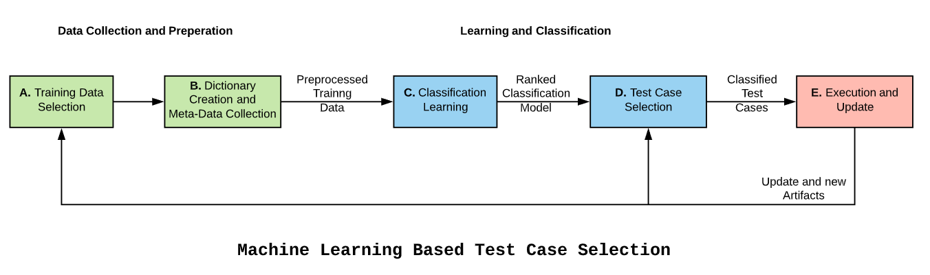
Data Collection and Preparation

For POC we have considered microservices Test cases across four release cycles as our Test Data.

This is an authorization microservice it is based on Oauth2 standard which is widely used in industry for authorization across systems/microservices. Refer this link for more information on Oauth2

Before going forward let’s understand how currently test selection process is happening in HP Cloud Print Platform

This image is specific to a particular organization but across the industry, the process is somewhat similar to this

Release Manifest: It is collection of versioned stuff that is being deployed, configuration settings, and issues/stories/artifacts description which are going to be deployed in particular release.

JIRA: Agile Project Management and Bug Tracking Tool.

Service Functionality Mapping File: Matrix which consists of mapping between Microservices and functionality , this will help users to understand impacted area when particular microservice getting affected.

Test Rail: Test Management Tool.

Let’s understand the process step by step

Step 1: For every release Subject Matter Expert(SME) refer Release Manifest to understand which microservices are under test and details of the fixes/commits in that particular release

Step 2: SME will take stories and Bug ID’s from Release Manifest and navigate to JIRA to get more relevant details , also based on the domain knowledge SME will refer Service Functionality Mapping File to understand impacted functionality

Step 3: Based on the information from JIRA ,SME will again refer Service Functionality Mapping File to get the list of impacted fucntionality

Step 4: Based on the impacted functionality list from above two steps SME will now navigate to Test Rail to search relevant test cases

Step 5: With the help of domain knowledge and data collected from above steps SME will select the list of test cases from Test Rail

Let’s take a quick look at test data which consists of regression test cases across four release cycles

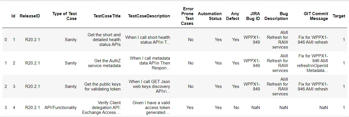
Let’s understand the columns/features present in dataset

ID: Unique Identifier of Records

ReleaseID : Release Identification number , Ex: R20.2.1 stands for ‘First release of 2 month of Year 2020

Type of Test Case : Cateogarization of Test cases , Ex: ‘Sanity’ test cases are supposed to be executed for Sanity of microservice and ‘API/Functionality’ test cases are for core functionality of microservice

TestCaseTitle : Title or summary of test case

TestCaseDescription : Steps for a test cases in Behavior Driven Devlopment(BDD) format

Error Prone Test Cases : Test cases which are covering high error prone area , these test cases must be executed in every release

Automation Status : Wheather test case is automated or not

Any Defect : If there is any defect in the release manifest then it will be mapped to the corresponding/relevant test cases and this column will be marked as ‘Yes’

JIRA Bug ID : Corresponding Bug ID of JIRA

Bug Description : JIRA Title/description of corresponding bug

GIT Commit Message : For particular release , if there are any commits in GIT then the corresponding/relevant test cases and this column will be marked with commit messages

Target : Binary classification of Test Cases selection

It’s quite possible that in actual , SME/Test Engineer is not considering above features/columns for test cases selection. But we strongly believe that these features should be considered during test case selection as they are directly or indirectly impacting Release and Qualification Cycles

Exploratory Data Analysis

Let’s explore these features one by one and it’s impact on target variable , in other words let’s try to understand how these features are related to selection of test cases. This analalysis will eventually help us in training our classifier model.

Let’s start with Categorical Variables ,will begin with ReleaseID.

We will check that how test cases are selected across different releases

#Getting unique value of releaseID column
dataset['ReleaseID'].unique()
dataset['ReleaseID'].value_counts()

R20.1.1     166
R19.12.1    166
R20.2.1     166
R20.1.2     166
Name: ReleaseID, dtype: int64

Test data comprise of four different releases and for each release there are equal number of test cases , but not all of them are selected for execution.

Let’s visualize that how many test cases selection is happening across release

It’s evident that selection of test cases is not uniform across the release and which is obvious , but we need to identify that what are the fetaures which play role in test case selection.

Let’s see how defects are mapped across releases

In R20.1.1 release there are 18 bugs and in R20.2.1 release there are 3 bugs , from the previous graph we can say that maximum number of selected test cases are in these two releases only .

With this analysis we can say that Any Defect feature is playing role in selection of test case.

Now let’s start exploring column Error Prone Test Cases

Number of Error Prone Test Cases is same in all release , on closer look it seems to be obvious because every release have similar set of test cases and these cases will be marked as ‘Error Prone’ based on domain expertise of SME.

Let’s see how these test cases are selected

printmd('**Number of Not Selected Error Prone Test Cases are {}**'.format(len(dataset[(dataset['Error Prone Test Cases'] == 'Yes') & (dataset['Target']=='No')].index)))

Number of Not Selected Error Prone Test Cases are 0

This means all Error Prone Test cases from each release are selected for executed , it means these cases are must executed test cases and this feature directly respobsible for selecting test cases

Let’s put our focus on another features Automation Status and Type of Test Case

First we will see what type of test cases are selected for executed

#Calculating total type of test cases
printmd("**Test Cases Segregation \n{}**".format(dataset['Type of Test Case'].value_counts()))

Test Cases Segregation:

API/Functionality	Integration	Sanity
640	12	12

All Sanity and Integration type of test cases are selected in all four release. With this we can conclude that Type of Test Cases are directly related to selection of test cases.

Now we will check Automation Status feature , will try to understand that how test cases are selected across releases based on automation status

• Total Number of Automated Test Cases are 236
• Total number of selected test cases which are automated 139

In our data set we have total 236 automated test cases and out of which 139 are selected test cases. Number of automated test cases are same in all four releases which is 59 .

Above data tell us that though number of automation test cases are same across all releases , selection of the same may depends upo other factors.

Let’s find out more how many automated test cases are selected in different releases

Highest number of automated selected test cases i.e 42% , 41% are in R20.1.1 and R20.2.1 releases respectively and from our pevious analysis we can say that these are the two releases where we have maximum number of bugs and highest number selected test cases.

With this it’s evident that Automation Test Cases feature played a role in test case selection specially when we have lot to test.

Above EDA looks obvious to many but the intent is to establish a relationship between features and target variable, so that classifier can learn the same pattern

With this we are done with analysis of all categorical data columns present in our data set and all of them looks related to our Target Variable , we will keep all of them in our further analysis.

Let’s start with Textual columns , we have following Text columns

1. Test Case Title
2. Test Case Description
3. JIRA Bug ID
4. Bug Description
5. GIT Commit Message

From above features list we can remove ‘JIRA Bug ID’ from our analysis because this is just a alphanumeric respresentation of Bugs and more details are present in next feature ‘Bug Description’.

Also , in our data set ‘GIT commit Message’ is very inconsistent and most of the commit messages are of bug fixing and for these fixes commit messages are either bug ID or bug description which is kind of duplicate of data present in feature ‘Bug Description’. We can drop GIT commit message column also.

It’s recommended that ‘Commit Messages’ should be there for test cases selection but for this relevant messages should enter at the time of commit and same has to be captured properly in Release Manifest for each releases

Let’s start looking at ‘Test Case Title’ and ‘Test Case Description’

There are no empty records in Test Case Title but same is not true for Description , majority of the description is empty.

Moreover , if we take a closer look in Title then we can say that it consist of summary of a test case which itself is a good information to select or unselect the test case. With this information we can drop ‘Test Case Description’ from our list.

Our Textual feature list for analysis will be reduced to following

1. Test Case Title
2. Bug Description

‘Test Case Title’ should be primary entry point for test cases selection as it give summary/intention behind the test case and this makes perfect choice for Test Case Selection

We have already concluded that ‘Any Defect’ column has direct relation with test case selection and if ‘Any Defect’ column has a value then corresponding ‘Bug Description’ should be there. With this co relation we can say that this column should be there in our feature list but in our data set only few entries are there fo ‘Bug Description’ , so we can skip this column also from our list

printmd("**Number of records with bug descriptions are {}**".format(len(dataset[pd.notnull(dataset["Bug Description"])].index)))

Number of records with bug descriptions are 21

#Drop not required column
dataset=dataset.drop(['TestCaseDescription','GIT Commit Message','JIRA Bug ID','Bug Description'],axis=1)
dataset.head()

	Id	ReleaseID	Type of Test Case	TestCaseTitle	Error Prone Test Cases	Automation Status	Any Defect	Target
0	1	R20.2.1	Sanity	Get the short and detailed health status APIs	No	Yes	Yes	1
1	2	R20.2.1	Sanity	Get the AuthZ service metadata	No	Yes	Yes	1
2	3	R20.2.1	Sanity	Get the public keys for validating token	No	Yes	Yes	1
3	4	R20.2.1	API/Functionality	Verify Client delegation API: Exchange Access ...	Yes	Yes	No	1
4	5	R20.2.1	API/Functionality	Verify Client delegation API:Exchange Access t...	No	Yes	No	1

Now, we have one text column and five categorical columns and based on our analysis we can say that all of these are related to selection of test cases i.e. related to ‘Target’ variable.

We can freeze above list of features for training classifier models , But before that we need to convert all categorical variables to encoded variables form and text columns into sparse matrix for features

#Encoding all categorical variable
from sklearn.preprocessing import LabelEncoder, OneHotEncoder
labelencoder = LabelEncoder()
dataset['ReleaseID']=labelencoder.fit_transform(dataset['ReleaseID'])
dataset['Error Prone Test Cases']=labelencoder.fit_transform(dataset['Error Prone Test Cases'])
dataset['Type of Test Case']=labelencoder.fit_transform(dataset['Type of Test Case'])
dataset['Automation Status']=labelencoder.fit_transform(dataset['Automation Status'])
dataset['Any Defect']=labelencoder.fit_transform(dataset['Any Defect'])
dataset.head()

	Id	ReleaseID	Type of Test Case	TestCaseTitle	Error Prone Test Cases	Automation Status	Any Defect	Target
0	1	3	2	Get the short and detailed health status APIs	0	1	1	1
1	2	3	2	Get the AuthZ service metadata	0	1	1	1
2	3	3	2	Get the public keys for validating token	0	1	1	1
3	4	3	0	Verify Client delegation API: Exchange Access ...	1	1	0	1
4	5	3	0	Verify Client delegation API:Exchange Access t...	0	1	0	1

With this all categorical columns are encoded into numerical values. Now , let’s deal with our only Text column i.e. ‘TestCaseTitle’.

For this we will apply Natural Language Processing (NLP) to convert text data into features for classifier model

Let’s create Corpus from ‘TestCaseTitle’ , Corpus is a simplified version of our test case title data that contain clean text data.

To create Corpus we have to perform the following actions

1. Remove unwanted words: Removal of unwanted words such as special characters and numbers to get only pure text. We will do it by specify our pattern using re library
2. Transform words to lowercase: Transform words to lowercase because upper and lower case have diffirent ASCII codes
3. Remove stopwords:Stop words are usually the most common words in a language and they will be irrelevant in determining the nature
4. Stemming words:Stemming is the process of reducing words to their word stem, base or root form. We use stemming to reduce Bag of Words dimensionality

#Importing required libraries
import re
import nltk
from nltk.corpus import stopwords
from nltk.stem.porter import PorterStemmer
corpus_title = []
pstem = PorterStemmer()
for i in range(dataset['TestCaseTitle'].shape[0]):
    #Remove unwanted words
    text = re.sub("[^a-zA-Z]", ' ', dataset['TestCaseTitle'][i])
    #Transform words to lowercase
    text = text.lower()
    text = text.split()
    #Remove stopwords then Stemming it
    text = [pstem.stem(word) for word in text if not word in set(stopwords.words('english'))]
    text = ' '.join(text)
    #Append cleaned tweet to corpus
    corpus_title.append(text)
    
printmd("**Corpus created successfully**") 

Corpus created successfully

From above Corpus we will create Bag of Words , which is representation of text that describes the occurrence of words within a document. It involves two things:

• A vocabulary of known words
• A measure of the presence of known words

This is called Bag of Word because any information about the order or structure of words in the document is discarded and the model is only concerned with whether the known words occur in the document, not where they occur in the document.

For Example :

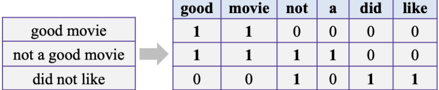
We can do this using scikit-learn’s CountVectorizer, where every row will represent a different test case and every column will represent a different word.

Countvectorizer converts a collection of text documents to a matrix of token counts. It is important to note here that CountVectorizer comes with a lot of options to automatically do preprocessing, tokenization, and stop word removal.However, i did all the process manually above to just get a better understanding.

# Creating the Bag of Words model
from sklearn.feature_extraction.text import CountVectorizer
cv = CountVectorizer()
text_vectors= cv.fit_transform(corpus_title).toarray()

#Convert text vectors into data frame
text_vectors_df=pd.DataFrame(text_vectors)
printmd("**Dimension for Text features are {}**".format(text_vectors_df.shape))

Dimension for Text features are (664, 115)

#Getting Target variable into Y variable
y=dataset[['Target']].values
#Converting 2 dimensional y and y_pred array into single dimension
y=y.ravel()

#Removing 'Target' and 'TestCaseTitle' columns from actual dataset
dataset=dataset.drop(['Target','TestCaseTitle'],axis=1)

#Creating new data frame with all categorical feature and Text features for training classifier models
X=pd.concat([dataset,text_vectors_df],axis=1).values
printmd("**Dimension for features data frame are {}**".format(X.shape))
#X.head()

Dimension for features data frame are (664, 121)

With this we have completed our EDA and Feature Engineering , let’s start with classifier models creation

Learning and Classification

Now we will build our models, for current data set we are using follwoing models

• Logistic Regression Model
• Gaussian Naive Bayes Model
• Multinomial Naive Bayes Model

If we have large data set we can use following models but for current data set we are avoiding them

• Decision Tree Model
• Gradient Boosting Model
• K - Nearest Neighbors Model

After building models we will evaluate our model based on confusion matrix , which is formed from the four outcomes produced as a result of binary classification

A binary classifier predicts all data instances of a test dataset as either positive or negative. This classification (or prediction) produces four outcomes — true positive, true negative, false positive and false negative.

• True positive (TP): correct positive prediction
• False positive (FP): incorrect positive prediction
• True negative (TN): correct negative prediction
• False negative (FN): incorrect negative prediction

A confusion matrix of binary classification is a two by two table formed by counting of the number of the four outcomes of a binary classifier. We usually denote them as TP, FP, TN, and FN instead of “the number of true positives”, and so on

Error rate (ERR) is calculated as the number of all incorrect predictions divided by the total number of the dataset. The best error rate is 0.0, whereas the worst is 1.0

Accuracy (ACC) is calculated as the number of all correct predictions divided by the total number of the dataset. The best accuracy is 1.0, whereas the worst is 0.0. It can also be calculated by 1 – ERR

F1 Score

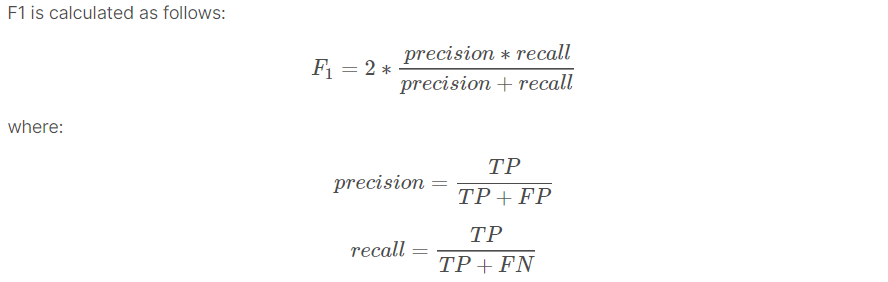
Based on above formulas we can evaluate our models in Train and Test data set

1. Regression Classifier F1 Score is 68.6
2. MultinomialNB Classifier F1 Score is 70.1
3. GaussianNB Classifier F1 Score is 70.1

Last Word

• Prediction could be improved if we have large data set , becuase then we can apply models like Decision Tree Model ,Gradient Boosting Model and K-Nearest Neighbors Model . We have checked these models for larger data set and prediction was pretty good
• Training data can be increase by adding more releases data
• Above approach can be used as a reference for similar problem statement

Note : I have captured very less code snippet for this blog , if interested in actual work then refer this notebook

Disclaimer: Just to let you know, this blog post was originally published on Medium. If you’d like to check out the original, you can find it at this link.